Webcam Calibration Check: How to Verify Accuracy

• Introduction
• Step-by-Step Guide
• Code Example
• Additional Notes
• Summary
• Conclusion
• References

Camera calibration is crucial for accurate computer vision applications, ensuring that your camera's lens distortions are corrected and measurements are reliable. Here are several methods to evaluate the success of your camera calibration:

1. Visual Comparison: Capture an image with your webcam and undistort it using the calibration parameters. Visually compare the distorted and undistorted images. Straight lines in the real world should appear straight in the undistorted image.

   # Assuming you have calibration parameters in 'mtx' and 'dist'
   undistorted_img = cv2.undistort(distorted_img, mtx, dist)

2. Reprojection Error: This method requires knowing the 3D world coordinates of points in your calibration pattern. After calibration, project the 3D points onto the image plane and compare them to their corresponding 2D points detected during calibration. The average distance between these points is the reprojection error. Lower error indicates better calibration.

3. Calibration Pattern Size and Border: Use the largest possible calibration pattern with a sufficient white border. This helps in accurate corner detection.

4. Camera Extrinsics Visualization: Tools like MATLAB's showExtrinsics function can visualize the camera's position and orientation relative to the calibration pattern. This helps in understanding if the camera poses during calibration were diverse enough.

5. Real-world Measurements: Place an object of known size in the camera's field of view. After calibration, measure the object's size in the undistorted image and compare it to its actual size. This provides a practical check on calibration accuracy.

6. Color Calibration: Use tools like Spyder Checkr to ensure consistent color representation across different cameras and lenses.

Remember that camera calibration is specific to a particular camera and lens combination. If you change either, you'll need to recalibrate.

This code demonstrates camera calibration and validation techniques using OpenCV in Python. It covers visual comparison of distorted and undistorted images, reprojection error calculation, calibration pattern size and border considerations, camera extrinsics visualization using matplotlib, real-world measurements for validation, and color calibration using tools like Spyder Checkr. The code provides examples for each technique, including loading calibration parameters, undistorting images, calculating reprojection error, visualizing camera poses, and measuring objects in undistorted images. It emphasizes the importance of recalibration when changing lenses or camera settings.

This code provides examples for several camera calibration validation techniques using OpenCV in Python.

1. Visual Comparison of Distorted and Undistorted Images:

import cv2

# Load calibration parameters
with np.load('calibration_parameters.npz') as file:
    mtx, dist = [file[i] for i in ('mtx', 'dist')]

# Capture image from webcam
cap = cv2.VideoCapture(0)
ret, frame = cap.read()
cap.release()

# Undistort the image
h,  w = frame.shape[:2]
newcameramtx, roi = cv2.getOptimalNewCameraMatrix(mtx, dist, (w,h), 1, (w,h))
undistorted_img = cv2.undistort(frame, mtx, dist, None, newcameramtx)

# Display distorted and undistorted images
cv2.imshow('Distorted Image', frame)
cv2.imshow('Undistorted Image', undistorted_img)
cv2.waitKey(0)
cv2.destroyAllWindows()

2. Reprojection Error Calculation:

import cv2
import numpy as np
import glob

# Load calibration parameters
with np.load('calibration_parameters.npz') as file:
    mtx, dist, rvecs, tvecs = [file[i] for i in ('mtx','dist','rvecs','tvecs')]

# Define criteria for corner refinement
criteria = (cv2.TERM_CRITERIA_EPS + cv2.TERM_CRITERIA_MAX_ITER, 30, 0.001)

# Prepare object points
objp = np.zeros((6*9,3), np.float32)
objp[:,:2] = np.mgrid[0:9,0:6].T.reshape(-1,2)

# Arrays to store object points and image points from all images
objpoints = [] 
imgpoints = [] 

# Load images of the calibration pattern
images = glob.glob('calibration_images/*.jpg')

for fname in images:
    img = cv2.imread(fname)
    gray = cv2.cvtColor(img, cv2.COLOR_BGR2GRAY)

    # Find the chessboard corners
    ret, corners = cv2.findChessboardCorners(gray, (9,6), None)

    # If found, add object points, image points (after refining them)
    if ret == True:
        objpoints.append(objp)
        corners2 = cv2.cornerSubPix(gray,corners, (11,11), (-1,-1), criteria)
        imgpoints.append(corners2)

# Calculate reprojection error
mean_error = 0
for i in range(len(objpoints)):
    imgpoints2, _ = cv2.projectPoints(objpoints[i], rvecs[i], tvecs[i], mtx, dist)
    error = cv2.norm(imgpoints[i], imgpoints2, cv2.NORM_L2)/len(imgpoints2)
    mean_error += error

print(f"Total error: {mean_error/len(objpoints)}")

3. Calibration Pattern Size and Border:

• Use a calibration pattern with a high number of corners (e.g., 9x6 or larger).
• Ensure a sufficient white border around the pattern for accurate corner detection.

4. Camera Extrinsics Visualization (using matplotlib):

import cv2
import numpy as np
import matplotlib.pyplot as plt
from mpl_toolkits.mplot3d import Axes3D

# Load calibration parameters
with np.load('calibration_parameters.npz') as file:
    mtx, dist, rvecs, tvecs = [file[i] for i in ('mtx','dist','rvecs','tvecs')]

# Define the 3D points of the calibration pattern
objp = np.zeros((6*9,3), np.float32)
objp[:,:2] = np.mgrid[0:9,0:6].T.reshape(-1,2)

# Create a figure and an axes object for the 3D plot
fig = plt.figure()
ax = fig.add_subplot(111, projection='3d')

# Plot the camera positions and orientations
for i in range(len(rvecs)):
    # Convert rotation vector to rotation matrix
    R, _ = cv2.Rodrigues(rvecs[i])
    
    # Get the camera position in world coordinates
    camera_position = -np.dot(R.T, tvecs[i])

    # Plot the camera position
    ax.scatter(camera_position[0], camera_position[1], camera_position[2], c='r', marker='o')

    # Plot the camera orientation
    arrow_length = 0.5
    ax.quiver(camera_position[0], camera_position[1], camera_position[2], 
              R[0, 0] * arrow_length, R[1, 0] * arrow_length, R[2, 0] * arrow_length, 
              color='r')
    ax.quiver(camera_position[0], camera_position[1], camera_position[2], 
              R[0, 1] * arrow_length, R[1, 1] * arrow_length, R[2, 1] * arrow_length, 
              color='g')
    ax.quiver(camera_position[0], camera_position[1], camera_position[2], 
              R[0, 2] * arrow_length, R[1, 2] * arrow_length, R[2, 2] * arrow_length, 
              color='b')

# Plot the calibration pattern
ax.scatter(objp[:, 0], objp[:, 1], objp[:, 2], c='b', marker='.')

# Set the axis labels and title
ax.set_xlabel('X')
ax.set_ylabel('Y')
ax.set_zlabel('Z')
ax.set_title('Camera Poses and Calibration Pattern')

# Display the plot
plt.show()

5. Real-world Measurements:

1. Place an object of known size (e.g., a ruler) in the camera's view.
2. Capture an image and undistort it using the calibration parameters.
3. Measure the object's size in the undistorted image using pixel coordinates.
4. Convert pixel measurements to real-world units using a known reference object or distance.
5. Compare the measured size with the actual size of the object.

6. Color Calibration:

• Use a color calibration target like Spyder Checkr to capture images with consistent colors.
• Software like SpyderX Pro can generate color profiles for your camera and lens combination.

Remember to recalibrate your camera whenever you change the lens or make significant adjustments to the camera settings.

General:

• Iteration is Key: Don't expect perfect calibration on the first try. Experiment with different settings, patterns, and environments to achieve the best results.
• Calibration Target Matters: The quality and type of your calibration pattern significantly impact accuracy. Consider professional targets for demanding applications.
• Environment Control: Consistent lighting and minimal reflections during both calibration and application are crucial for reliable results.

Specific to Methods:

• Visual Comparison: While a good starting point, this method is subjective. What looks straight to one person might not to another. Use objective measures whenever possible.
• Reprojection Error:
  • Aim for a reprojection error less than 1 pixel for ideal results.
  • Error distribution matters. Consistently high errors in specific image regions might indicate lens distortion the calibration struggles to correct.
• Camera Extrinsics Visualization:
  • Ensure good coverage. The calibration pattern should be viewed from various angles and distances to capture the full range of lens behavior.
  • Look for clustered camera poses. This suggests limited variation in calibration images, potentially leading to poor generalization.
• Real-world Measurements:
  • Use multiple objects and distances for a more comprehensive assessment.
  • Consider the accuracy of your real-world measurements. Small errors in measurement can propagate and skew your calibration validation.
• Color Calibration:
  • Important for applications where color accuracy is critical, such as color-based object tracking or medical imaging.
  • Keep in mind that color calibration might require specialized hardware and software.

Beyond the Basics:

• Tangential Distortion: The provided code examples focus on radial distortion. For high-accuracy applications, consider calibrating for tangential distortion as well.
• Dynamic Environments: If your application involves moving cameras or changing environments, explore online or continuous calibration techniques.
• Specialized Calibration: For specific camera models or applications like multi-camera systems, research specialized calibration procedures and tools.

This article outlines several methods to evaluate the success of your camera calibration:

Visual Inspection:

• Undistortion: Apply undistortion to a captured image and visually compare it to the original. Straight lines in the real world should appear straight in the undistorted image.
• Extrinsics Visualization: Use tools like MATLAB's showExtrinsics to visualize the camera's position and orientation during calibration. This helps ensure diverse camera poses.

Quantitative Metrics:

• Reprojection Error: Calculate the average distance between projected 3D points (from your calibration pattern) and their corresponding 2D points detected in the image. Lower error indicates better calibration.
• Real-world Measurements: Measure a known-size object in the undistorted image and compare it to its actual size. This provides a practical accuracy check.

Calibration Best Practices:

• Pattern Optimization: Use the largest possible calibration pattern with a sufficient white border for accurate corner detection.
• Color Calibration: Employ tools like Spyder Checkr to ensure consistent color representation across different cameras and lenses.

Important Note: Camera calibration is specific to a particular camera and lens combination. Recalibration is necessary if either component changes.

In conclusion, thoroughly validating your camera calibration is essential for achieving accurate results in computer vision applications. Employing a combination of visual checks, quantitative metrics like reprojection error and real-world measurements, and adhering to best practices during calibration ensures your camera system is reliable and your vision applications are successful. Remember that calibration is not a one-time process; it's crucial to recalibrate whenever significant changes occur, such as changing the lens or altering the camera's environment.

• How to verify the correctness of calibration of a webcam - OpenCV ... | Oct 9, 2012 ... A versatile camera calibration technique for high accuracy 3d machine vision metrology using off-the-shelf tv cameras and lenses.
• computer vision - How to verify that the camera calibration is correct ... | Aug 5, 2013 ... The quality of calibration is measured by the reprojection error (is there an alternative?), which requires a knowledge world coordinates of some 3d point(s).
• How do I get the most accurate camera calibration? | Feb 26, 2012 ... Make sure you have the largest possible calibration pattern. · Make sure your printed pattern has enough white border around it, otherwise it may ...
• matlab - Verify that camera calibration is still valid - Stack Overflow | Jul 22, 2015 ... If you have a single camera you can easily follow the steps from this article: Evaluating the Accuracy of Single Camera Calibration.
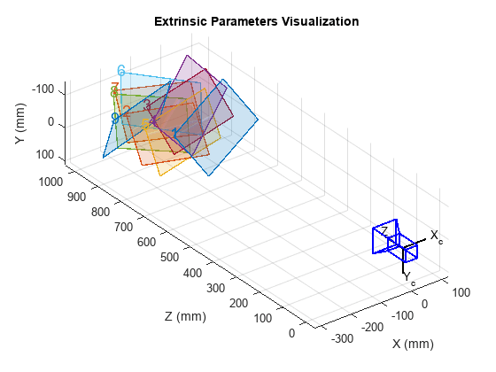• Evaluating the Accuracy of Single Camera Calibration | Use the showExtrinsics function to either plot the locations of the calibration pattern in the camera's coordinate system, or the locations of the camera in the ...
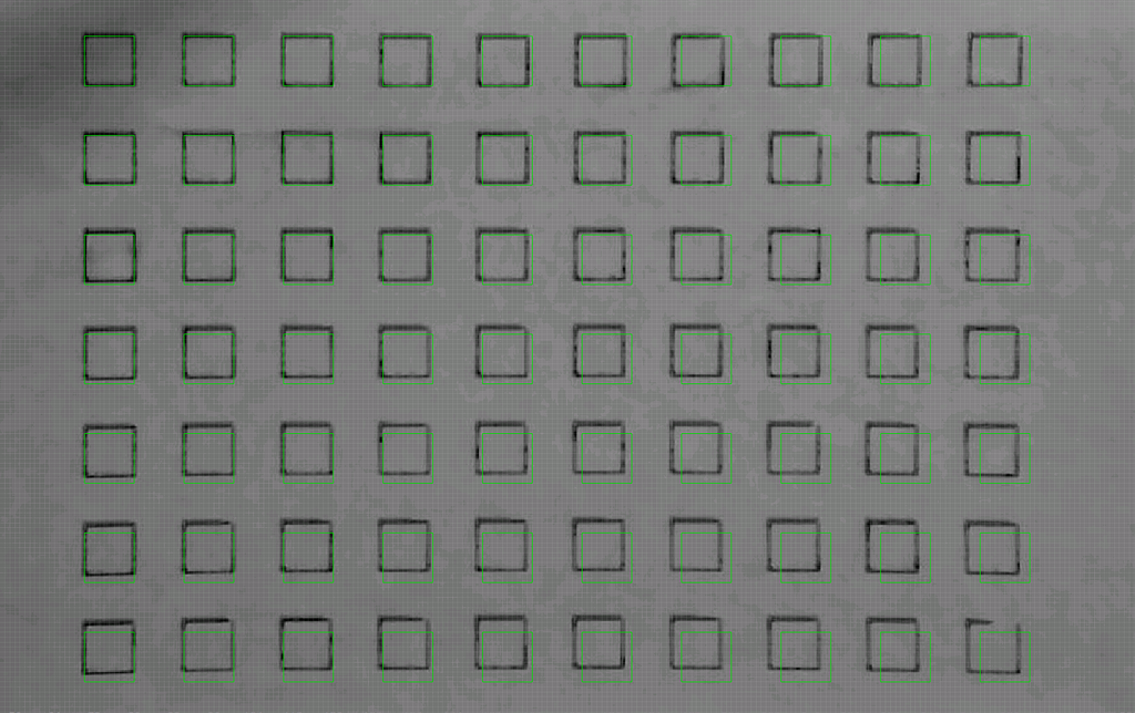• Camera Alignment Accuracy - LightBurn Software Questions ... | I have two questions related to the accuracy of camera alignment; I will first describe the context. I have integrated the Atomstack AC1, a 5MP camera (I am considering an 8MP camera) During the calibration, all scores were below 0.2, a good sign Before aligning, I have reduced the Working Area to (300, 300) (During the first iterations, I have kept the original (430, 400) Working Area, the results were similar to what is described below) During the alignment, I have set Scale to 150 (1.5*20...
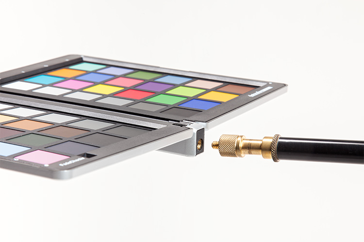• Spyder Checkr - Datacolor Spyder | ... calibrate all your cameras, so camera-to-camera matching, accuracy and printability are easy. Color can also vary from lens to lens attached to the same ...
• LightBurn Camera Features - what accuracy does it offer ... | Good afternoon, I looked for this answer in other posts but I couldn’t find it. My first question is: lightburn doesn’t male automatic cut registration/alignment using camera detectable registration marks, right? (like ruida’s sv300 camera does in RD Works, for example) My second question: with Ligthburn’s official camera, with 4k resolution, what precision can I get on a 60x40cm table? Thank you for the help
• Cannot get good camera calibration - OpenCV | Hello, I am trying to do a basic calibration of my two USB cameras, with little success so far. I am using a 9x14 corner chessboard, with each image at 1080p, and tried different sets of calibration data, but no matter what I try my undistorted image always looks a fair bit worse than the original, and the ret value given by cv2.calibrateCamera() is over 100, which if I understand correctly is quite large. At the same time, looking at the results of the cv2.drawChessboardCorners() function, all ...