Disparity Map Definition: Understanding Depth Perception

• Introduction
• Step-by-Step Guide
• Code Example
• Additional Notes
• Summary
• Conclusion
• References

A disparity map is like a magic lens that reveals depth in a pair of images. Imagine you have two eyes, each capturing a slightly different view of the world. Your brain effortlessly combines these images to perceive depth. A disparity map does something similar. It starts with two images taken from slightly different angles, like those from a stereo camera. The map itself is a grayscale image where each pixel value represents the difference in position of a corresponding point in the two images. Brighter pixels in the disparity map indicate objects closer to the camera, while darker pixels represent objects farther away. This is because closer objects have a larger difference in their positions between the two images. Think of it like this: hold your finger close to your face and close one eye, then switch eyes. Your finger seems to jump a greater distance than objects in the background. This jump is what the disparity map captures. Disparity maps are crucial for various applications, including 3D reconstruction, depth estimation, and even robot navigation. By analyzing the differences in pixel positions, we can infer depth information and understand the spatial relationships between objects in a scene.

A disparity map is like a magic lens that reveals depth in a pair of images. Imagine you have two eyes, each capturing a slightly different view of the world. Your brain effortlessly combines these images to perceive depth. A disparity map does something similar.

left_image = cv2.imread('left.png')
right_image = cv2.imread('right.png')

It starts with two images taken from slightly different angles, like those from a stereo camera. The map itself is a grayscale image where each pixel value represents the difference in position of a corresponding point in the two images.

stereo = cv2.StereoBM_create()
disparity_map = stereo.compute(left_image, right_image)

Brighter pixels in the disparity map indicate objects closer to the camera, while darker pixels represent objects farther away. This is because closer objects have a larger difference in their positions between the two images.

plt.imshow(disparity_map, 'gray')
plt.show()

Think of it like this: hold your finger close to your face and close one eye, then switch eyes. Your finger seems to jump a greater distance than objects in the background. This jump is what the disparity map captures.

Disparity maps are crucial for various applications, including 3D reconstruction, depth estimation, and even robot navigation. By analyzing the differences in pixel positions, we can infer depth information and understand the spatial relationships between objects in a scene.

This Python code uses OpenCV and matplotlib libraries to compute and visualize a disparity map from a pair of rectified stereo images. It loads the left and right images, creates a StereoBM object, computes the disparity map, normalizes it for display, and finally shows the disparity map using matplotlib.

import cv2
import matplotlib.pyplot as plt

# Load the left and right stereo images
left_image = cv2.imread('left.png', cv2.IMREAD_GRAYSCALE)
right_image = cv2.imread('right.png', cv2.IMREAD_GRAYSCALE)

# Create a StereoBM object for computing the disparity map
stereo = cv2.StereoBM_create(numDisparities=16, blockSize=15)

# Compute the disparity map
disparity_map = stereo.compute(left_image, right_image)

# Normalize the disparity map for display
disparity_map = cv2.normalize(disparity_map, None, 255,0, cv2.NORM_MINMAX, cv2.CV_8U)

# Display the disparity map
plt.imshow(disparity_map, 'gray')
plt.title('Disparity Map')
plt.show()

Explanation:

1. Import Libraries: Import the necessary libraries, cv2 for OpenCV and matplotlib.pyplot for plotting.
2. Load Images: Load the left and right stereo images using cv2.imread(). Make sure to load them as grayscale images using the cv2.IMREAD_GRAYSCALE flag.
3. Create StereoBM Object: Create a cv2.StereoBM_create() object. This object is responsible for computing the disparity map using the block matching algorithm. You can adjust parameters like numDisparities (number of disparities to consider) and blockSize (size of the blocks for matching) for better results depending on your images.
4. Compute Disparity Map: Use the stereo.compute() method to calculate the disparity map from the left and right images.
5. Normalize Disparity Map: The disparity map values are typically in a large range. Normalize them to the 0-255 range using cv2.normalize() for better visualization.
6. Display Disparity Map: Finally, display the disparity map using plt.imshow() from matplotlib.

Key Points:

• Stereo Images: You need a pair of stereo images taken from slightly different viewpoints for this code to work.
• Image Alignment: The images should be rectified beforehand, meaning any lens distortion should be corrected, and the images should be aligned so that corresponding points lie on the same horizontal line.
• Parameter Tuning: The numDisparities and blockSize parameters of cv2.StereoBM_create() can significantly affect the quality of the disparity map. Experiment with different values to find what works best for your images.

This code provides a basic example of disparity map generation. You can explore more advanced stereo matching algorithms and techniques for improved accuracy and robustness in real-world applications.

• Disparity Range: The disparity values usually fall within a specific range, often determined by the numDisparities parameter during StereoBM object creation. Understanding this range is important for interpreting the disparity map correctly.
• Occlusion Handling: Areas in one image that are not visible in the other (due to object occlusion) will result in invalid disparity values. These areas often appear as black regions or holes in the disparity map.
• Smoothing and Filtering: The raw disparity map might contain noise or artifacts. Applying smoothing filters (like median filters) can help reduce noise and improve the visual quality of the map.
• Real-Time Applications: For real-time applications like robot navigation, efficient stereo matching algorithms and hardware acceleration are crucial to achieve the necessary processing speed.
• Alternative Algorithms: StereoBM is a basic block matching algorithm. More sophisticated algorithms like Semi-Global Block Matching (SGBM) and dynamic programming-based approaches can provide more accurate disparity maps, especially at object boundaries and in textured regions.
• Depth Calculation: The disparity map can be converted to a depth map using camera parameters (focal length, baseline distance between cameras). The depth map provides actual distance measurements to objects in the scene.
• Applications Beyond Vision: Disparity maps have applications beyond traditional computer vision, such as in medical imaging (stereo endoscopy) and remote sensing (stereo aerial imagery).
• Limitations: Disparity map generation can be challenging in scenes with low texture, repetitive patterns, specular reflections, or significant lighting variations between the stereo images.

This article explains the concept of a disparity map and its use in depth perception.

Here's a summary:

• What it is: A disparity map is a grayscale image that reveals depth information from two images taken from slightly different angles (like human eyes).
• How it works: Each pixel in the disparity map represents the difference in position of a corresponding point in the two input images.
  • Brighter pixels indicate objects closer to the camera (larger difference in position between images).
  • Darker pixels represent objects farther away (smaller difference in position).
• Analogy: Imagine closing one eye and then the other while focusing on your finger. The apparent "jump" your finger makes compared to the background illustrates the concept of disparity.
• Applications: Disparity maps are crucial for:
  • 3D reconstruction
  • Depth estimation
  • Robot navigation

In essence, disparity maps allow us to extract valuable depth information from images, enabling a deeper understanding of the spatial relationships within a scene.

In conclusion, disparity maps, generated from the subtle differences between two images, provide a powerful tool for extracting depth information. This grayscale representation, where brighter pixels signify proximity and darker ones indicate distance, finds applications in diverse fields like 3D modeling, robotic vision, and depth perception. By analyzing the "jumps" or disparities, we gain a deeper understanding of spatial relationships within a scene, essentially enabling machines to perceive depth much like human vision. As technology advances, the role of disparity maps in bridging the gap between 2D images and 3D understanding continues to expand, opening up new possibilities in various fields.

• Literature Survey on Stereo Vision Disparity Map Algorithms ... | This paper presents a literature survey on existing disparity map algorithms. It focuses on four main stages of processing as proposed by Scharstein and Szeliski in a taxonomy and evaluation of dense...
• java - How to create a disparity map? - Stack Overflow | Nov 22, 2011 ... I need to write this to a disparity map. The disparity maps I have found are grayscale images, with lighter grays meaning less depth and darker ...
• Disparity Map - an overview | ScienceDirect Topics | A disparity map computes the horizontal displacement in each pixel between two images. Wang et al. [57] present a technique for disparity estimation.
• computer vision - What is the difference between a disparity map ... | Jul 12, 2013 ... What is the definition of a "disparity map"? 1 · Finding the corresponding pixel using disparity maps · 9 · Stereo vision: Depth estimation · 6.
• Disparity Map | Historically, a disparity map is a visual representation of the differences in pixel coordinates between the corresponding points in a stereo image pair. It is typically generated from a pair of stereo images taken from slightly different viewpoints (left and right cameras). Using the power of the I...
• Understanding Depth Map / Depth Image / Disparity Map / Disparity ... | Feb 26, 2022 ... Can you provide a link within your question to the sources where you found the definitions and examples you refer to? ... Disparity Map: A ...
• Disparity Map in Stereo Vision | Baeldung on Computer Science | Explore the concept of disparity, and learn about its importance in stereo vision.
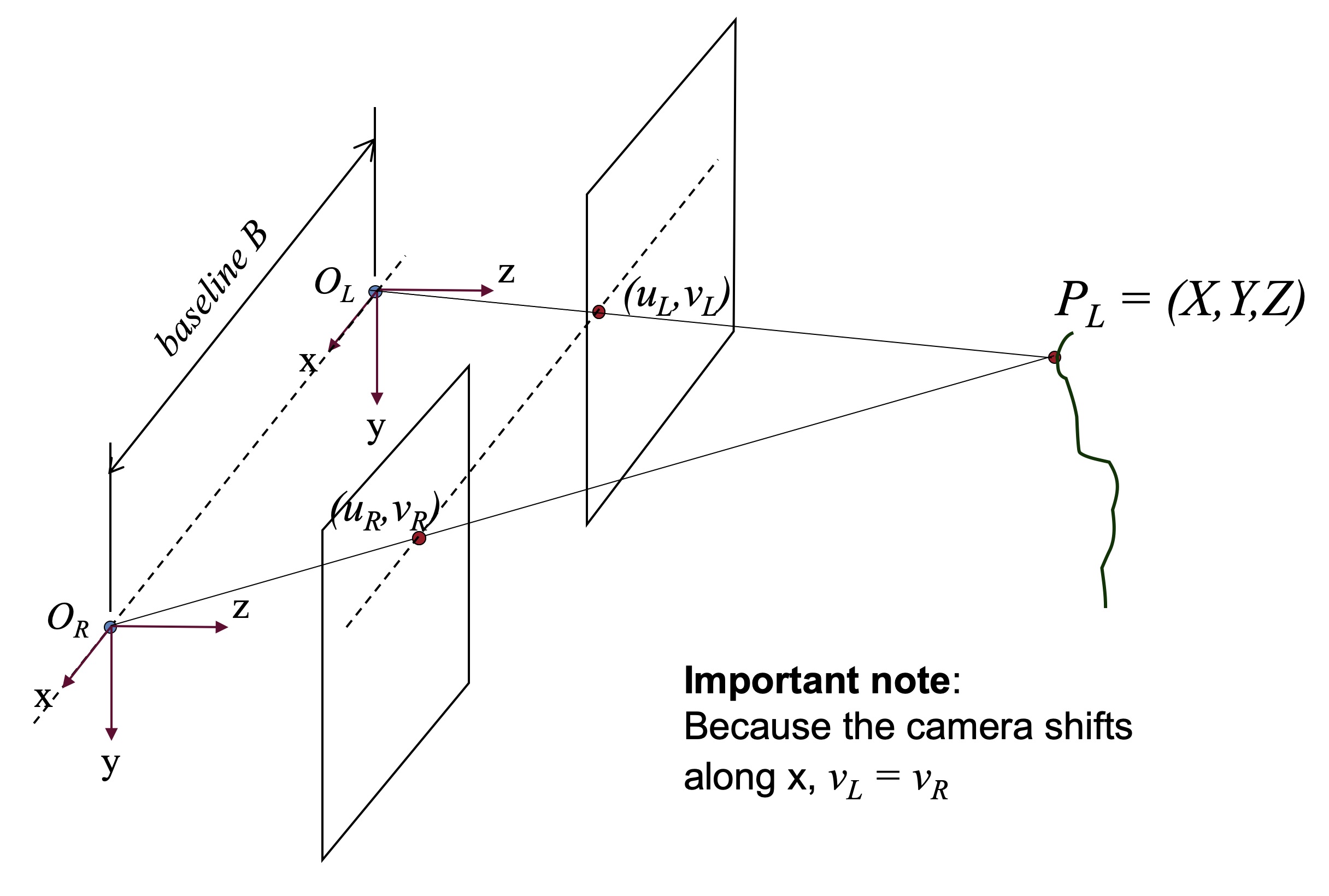• Stereo and Disparity | John Lambert | Dec 27, 2018 ... Stereo Geometry; Disparity; Classical Matching Techniques; A First Stereo Algorithm; Disparity Map; Cost Volumes; Smoothing; When is smoothing a ...
• disparity | Examples. collapse all. Compute Disparity Map for a Pair of Stereo Images. Open ... The function defines uniqueness as a ratio of the optimal disparity ...