In Keras, both UpSampling2D and Conv2DTranspose layers are utilized to increase the size of feature maps, a crucial operation in various deep learning tasks such as image segmentation and generative modeling. However, these layers differ significantly in their underlying mechanisms and resulting outputs.
Both UpSampling2D and Conv2DTranspose are used in Keras for increasing the size of feature maps, but they work differently:
UpSampling2D:
-
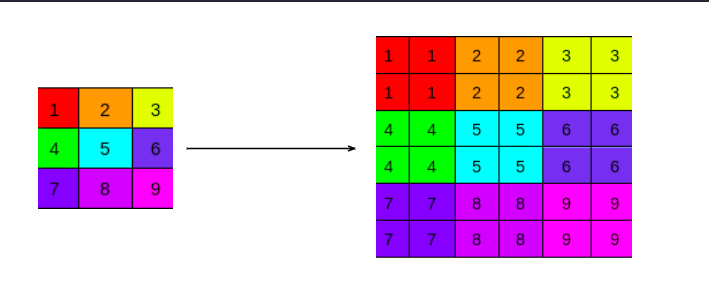
Simpler method: It simply repeats rows and columns to upscale.
from tensorflow.keras.layers import UpSampling2D
upsample = UpSampling2D(size=(2, 2))
-
Fast but less sophisticated: Can lead to blocky artifacts, especially if not followed by convolutional layers.
Conv2DTranspose:
-
Learnable upsampling: Uses a convolution operation (like
Conv2D) but in reverse to learn how to upsample.
from tensorflow.keras.layers import Conv2DTranspose
upsample = Conv2DTranspose(filters=32, kernel_size=(3, 3), strides=(2, 2), padding='same')
-
More powerful: Can learn smoother and more complex upsampling patterns.
-
Slower and more computationally expensive: Requires more parameters and computations.
In summary:
- Use
UpSampling2D for quick and basic upsampling, often followed by Conv2D for smoothing.
- Use
Conv2DTranspose when you need the model to learn the best upsampling method, especially in generative models like GANs.
This Python code demonstrates two methods for upsampling images using TensorFlow and Keras: UpSampling2D and Conv2DTranspose. It defines separate models for each method, provides a summary of their architectures, and includes an optional visualization to compare their outputs on a sample input image. The code highlights the key parameters and usage of both upsampling techniques, allowing for easy experimentation and understanding of their effects on image dimensions and feature maps.
import tensorflow as tf
from tensorflow.keras.layers import Input, UpSampling2D, Conv2DTranspose, Conv2D
from tensorflow.keras.models import Model

# Define input shape
input_shape = (8, 8, 3)  # Example: 8x8 image with 3 channels

# --- UpSampling2D Example ---
# Define input layer
inputs = Input(shape=input_shape)
# Upsample by a factor of 2 in both dimensions
upsampled = UpSampling2D(size=(2, 2))(inputs)
# Optional: Add a Conv2D layer for smoothing
# upsampled = Conv2D(filters=64, kernel_size=(3, 3), activation='relu', padding='same')(upsampled)
# Create the model
model_upsampling = Model(inputs, upsampled)

# --- Conv2DTranspose Example ---
# Define input layer
inputs = Input(shape=input_shape)
# Upsample and learn 32 feature maps
upsampled = Conv2DTranspose(filters=32, kernel_size=(3, 3), strides=(2, 2),
                           activation='relu', padding='same')(inputs)
# Create the model
model_transpose = Model(inputs, upsampled)

# --- Print Model Summaries ---
print("Model using UpSampling2D:")
model_upsampling.summary()

print("\nModel using Conv2DTranspose:")
model_transpose.summary()

# --- Visualize the Upsampling (Optional) ---
import numpy as np
import matplotlib.pyplot as plt

# Create a sample input image (replace with your own data)
sample_input = np.random.rand(1, *input_shape)

# Get the output of both models
output_upsampling = model_upsampling.predict(sample_input)
output_transpose = model_transpose.predict(sample_input)

# Display the results
plt.figure(figsize=(10, 5))

plt.subplot(1, 3, 1)
plt.title("Input")
plt.imshow(sample_input[0])

plt.subplot(1, 3, 2)
plt.title("UpSampling2D")
plt.imshow(output_upsampling[0, :, :, 0])  # Show the first channel

plt.subplot(1, 3, 3)
plt.title("Conv2DTranspose")
plt.imshow(output_transpose[0, :, :, 0])  # Show the first channel

plt.show()
Explanation:
-
Import Necessary Layers: Import
UpSampling2D, Conv2DTranspose, Conv2D, and other required layers.
-
Define Input: Create an
Input layer to specify the shape of your input data.
-
UpSampling2D Model:
- Create an
UpSampling2D layer with the desired size (upsampling factor).
- (Optional) Add a
Conv2D layer after upsampling to smooth out the results.
- Create a
Model using the input and output layers.
-
Conv2DTranspose Model:
- Create a
Conv2DTranspose layer, specifying:
-
filters: The number of output filters (feature maps).
-
kernel_size: The size of the convolution kernel.
-
strides: The upsampling factor (usually (2, 2) for doubling the size).
-
padding: 'same' to maintain the spatial dimensions.
- Create a
Model using the input and output layers.
-
Print Summaries: Use
model.summary() to see the architecture and parameters of both models.
-
Visualize (Optional):
- Create some sample input data.
- Use
model.predict() to get the upsampled outputs from both models.
- Use
matplotlib to display the input and the upsampled results for comparison.
Key Points:
- This code provides a clear comparison between
UpSampling2D and Conv2DTranspose for upsampling in Keras.
- You can easily modify the input shape, upsampling factors, and other parameters to experiment with different settings.
- The optional visualization part helps you see the difference in the upsampled outputs generated by the two methods.
-
Interpolation in UpSampling2D: While the default for UpSampling2D is nearest neighbor interpolation (simply repeating pixels), you can specify other interpolation methods like 'bilinear' for smoother results. However, this still won't be as powerful as learned upsampling with Conv2DTranspose.
-
Checkerboard Artifacts: Conv2DTranspose can sometimes introduce "checkerboard" artifacts in the upsampled output. This is often due to the kernel size and stride not aligning properly. Using techniques like "sub-pixel convolution" or carefully choosing kernel sizes can help mitigate this issue.
-
Applications Beyond Upsampling: While primarily used for upsampling in image generation, Conv2DTranspose can also be used in other contexts like:
-
Deconvolution: To visualize feature maps and understand what the network is learning.
-
Unsupervised Learning: In autoencoders for learning compressed representations and reconstructing data.
-
Parameter Efficiency: If you need to be mindful of model size and computational cost, UpSampling2D followed by Conv2D can be a more parameter-efficient way to achieve reasonable upsampling compared to Conv2DTranspose.
-
Experimentation is Key: The choice between UpSampling2D and Conv2DTranspose depends on the specific application and desired output quality. It's often beneficial to experiment with both methods and compare the results to determine the best option.
| Feature |
UpSampling2D |
Conv2DTranspose |
| Mechanism |
Repeats rows and columns |
Learns upsampling through convolution |
| Implementation |
UpSampling2D(size=(2, 2)) |
Conv2DTranspose(filters=32, kernel_size=(3, 3), strides=(2, 2), padding='same') |
| Output Quality |
Can be blocky, needs smoothing |
Smoother, learns complex patterns |
| Performance |
Fast and lightweight |
Slower and computationally expensive |
| Use Cases |
Quick upsampling, often followed by Conv2D
|
When learned upsampling is crucial, e.g., GANs |
In short: Choose UpSampling2D for speed and simplicity, and Conv2DTranspose for higher quality and learned upsampling.
While both UpSampling2D and Conv2DTranspose serve to increase feature map sizes in Keras, they employ distinct methods with differing outcomes. UpSampling2D provides a straightforward approach by replicating rows and columns, proving computationally efficient but potentially yielding less refined outputs. Conversely, Conv2DTranspose leverages a learnable upsampling mechanism through reverse convolution, enabling the acquisition of more sophisticated and smoother upsampling patterns, albeit at the cost of increased computational demands. The choice between these layers hinges on the specific application requirements. UpSampling2D proves suitable for rapid, rudimentary upsampling, often supplemented by Conv2D for smoothing, while Conv2DTranspose excels in scenarios demanding the model to ascertain optimal upsampling techniques, particularly in generative models like GANs. Ultimately, selecting the appropriate upsampling method necessitates a nuanced understanding of the trade-offs between output quality, computational efficiency, and the intricacies of the task at hand.
-
 Difference between UpSampling2D and Conv2DTranspose ... | A Computer Science portal for geeks. It contains well written, well thought and well explained computer science and programming articles, quizzes and practice/competitive programming/company interview Questions.
-
 How to use the UpSampling2D and Conv2DTranspose Layers in ... | Generative Adversarial Networks, or GANs, are an architecture for training generative models, such as deep convolutional neural networks for generating images. The GAN architecture is comprised of both a generator and a discriminator model. The generator is responsible for creating new outputs, such as images, that plausibly could have come from the original dataset. The […]
-
 Difference between Loss Function and Metric in Keras ... | Loss functions in Keras measure the error between predicted and actual values to optimize model training, while metrics evaluate and monitor model performance without directly influencing the training process.
-
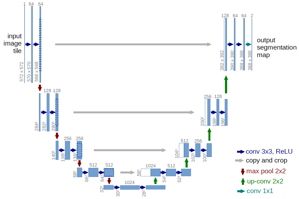 UpSampling2D vs Conv2DTranspose: U-Net Architecture | by ... | Introduction
-
 fft - Perform Transposed Convolution in Spectral / Frequency ... | Jul 1, 2021 ... ... in the context of Deep Learning the whole idea of ... What is the difference between UpSampling2D and Conv2DTranspose functions in keras?
-
 DigitalSreeni - YouTube | Welcome to my Python coding channel! Here, I'll teach you everything from the very basics to advanced topics in machine learning and deep learning. I'll focus a lot on image processing and other relevant topics.
How to cite my work?
YouTube video:
The general format for citing a YouTube video in APA (American Psychological Association) style is:
Author’s Last Name, First Initial. (Year, Month Day Published). Title of video [Video]. YouTube. URL
So, here is an example:
Bhattiprolu, S. (2023, August 23). 330 - Fine tuning Detectron2 for instance segmentation using custom data [Video]. YouTube. https://youtu.be/cEgF0YknpZw
GitHub code:
Author’s Last Name, First Initial. (Year). Title of Repository. GitHub. URL
Example:
Bhattiprolu, S. (2023). python_for_microscopists. GitHub. https://github.com/bnsreenu/python_for_microscopists/blob/master/330_Detectron2_Instance_3D_EM_Platelet.ipynb