Optical flow is a powerful technique in computer vision that analyzes the motion of pixels between consecutive images. It has two main variants: sparse and dense optical flow.
-
Optical flow analyzes how pixels move between image sequences, like in a video.
-
Sparse optical flow calculates this movement for a select few "interesting" pixels. Imagine tracking corners of a moving object.
# Example using OpenCV in Python
feature_params = dict( maxCorners = 100,
                    qualityLevel = 0.3,
                    minDistance = 7,
                    blockSize = 7 )
lk_params = dict( winSize  = (15,15),
                maxLevel = 2,
                criteria = (cv2.TERM_CRITERIA_EPS | cv2.TERM_CRITERIA_COUNT, 10, 0.03))
p0 = cv2.goodFeaturesToTrack(old_gray, mask = None, **feature_params)
p1, st, err = cv2.calcOpticalFlowPyrLK(old_gray, frame_gray, p0, None, **lk_params)
-
Dense optical flow computes the motion for every pixel in the image. Think of it like a detailed map of how everything shifted.
# Example using OpenCV in Python
flow = cv2.calcOpticalFlowFarneback(prvs, next, None, 0.5, 3, 15, 3, 5, 1.2, 0)
- Sparse is computationally cheaper and faster, ideal for tasks like tracking specific points.
- Dense is more detailed but requires more processing power. It's used for tasks like understanding scene depth or video segmentation.
- Algorithms like Lucas-Kanade are often used for sparse, while Farneback is common for dense optical flow.
- Recent advancements use deep learning to estimate optical flow, even from sparse data like event cameras.
- Choosing between sparse and dense depends on your application's needs for speed, accuracy, and the level of detail required.
This Python code demonstrates optical flow using OpenCV. It reads a video file and performs both sparse and dense optical flow calculations. Sparse optical flow is implemented using the Lucas-Kanade method, tracking the movement of specific feature points. Dense optical flow is calculated using the Farneback method, providing flow vectors for every pixel in the image. The results are visualized by drawing tracks for sparse optical flow and displaying a color-coded representation of the flow vectors for dense optical flow. The code iterates through the video frames, updating the calculations and visualizations for each frame.
import cv2
import numpy as np

# Load video
cap = cv2.VideoCapture('your_video.mp4')

# Take first frame and find corners in it
ret, old_frame = cap.read()
old_gray = cv2.cvtColor(old_frame, cv2.COLOR_BGR2GRAY)

# Parameters for ShiTomasi corner detection (for sparse optical flow)
feature_params = dict( maxCorners = 100,
                       qualityLevel = 0.3,
                       minDistance = 7,
                       blockSize = 7 )

# Parameters for Lucas-Kanade optical flow
lk_params = dict( winSize  = (15,15),
                  maxLevel = 2,
                  criteria = (cv2.TERM_CRITERIA_EPS | cv2.TERM_CRITERIA_COUNT, 10, 0.03))

# Create a mask image for drawing purposes
mask = np.zeros_like(old_frame)

# Find initial corner locations
p0 = cv2.goodFeaturesToTrack(old_gray, mask = None, **feature_params)

while(1):
    ret, frame = cap.read()
    if not ret:
        break
    frame_gray = cv2.cvtColor(frame, cv2.COLOR_BGR2GRAY)

    # -------------------- Sparse Optical Flow --------------------
    # Calculate sparse optical flow using Lucas-Kanade method
    p1, st, err = cv2.calcOpticalFlowPyrLK(old_gray, frame_gray, p0, None, **lk_params)

    # Select good points
    good_new = p1[st==1]
    good_old = p0[st==1]

    # Draw the tracks
    for i,(new,old) in enumerate(zip(good_new,good_old)):
        a,b = new.ravel()
        c,d = old.ravel()
        mask = cv2.line(mask, (a,b),(c,d), (0,0,255), 2)
        frame = cv2.circle(frame,(a,b),5,(0,0,255),-1)

    # -------------------- Dense Optical Flow --------------------
    # Calculate dense optical flow using Farneback method
    flow = cv2.calcOpticalFlowFarneback(old_gray, frame_gray, None, 0.5, 3, 15, 3, 5, 1.2, 0)

    # Visualize dense optical flow
    magnitude, angle = cv2.cartToPolar(flow[..., 0], flow[..., 1])
    mask_flow = np.zeros_like(frame)
    mask_flow[..., 1] = 255
    mask_flow[..., 0] = angle * 180 / np.pi / 2
    mask_flow[..., 2] = cv2.normalize(magnitude, None, 0, 255, cv2.NORM_MINMAX)
    rgb_flow = cv2.cvtColor(mask_flow, cv2.COLOR_HSV2BGR)

    # Display results
    img = cv2.add(frame, mask)
    cv2.imshow('Sparse Optical Flow', img)
    cv2.imshow('Dense Optical Flow', rgb_flow)

    # Update previous frame and points
    old_gray = frame_gray.copy()
    p0 = good_new.reshape(-1,1,2)

    k = cv2.waitKey(30) & 0xff
    if k == 27:
        break

cv2.destroyAllWindows()
cap.release()
Explanation:
-
Import Libraries: Import necessary libraries like
cv2 (OpenCV) and numpy.
-
Load Video: Load the video file using
cv2.VideoCapture().
-
Preprocess First Frame: Read the first frame and convert it to grayscale for optical flow calculations.
-
Sparse Optical Flow:
-
Feature Detection: Use
cv2.goodFeaturesToTrack() to find strong corners in the first frame. These will be the points tracked.
-
Lucas-Kanade Algorithm: Use
cv2.calcOpticalFlowPyrLK() to calculate the optical flow of the detected features between the current and previous frame.
-
Visualize Tracks: Draw lines on the image to visualize the movement of the tracked points.
-
Dense Optical Flow:
-
Farneback Algorithm: Use
cv2.calcOpticalFlowFarneback() to calculate the dense optical flow for the entire image.
-
Visualize Flow: Convert the flow vectors to HSV color space for visualization. The hue represents the direction of flow, and the value represents the magnitude.
-
Display Results: Display both the sparse and dense optical flow results in separate windows.
-
Update Loop: Update the previous frame and tracked points for the next iteration of the loop.
This code provides a basic example of how to implement both sparse and dense optical flow using OpenCV in Python. You can modify the parameters and visualization techniques to suit your specific needs.
Assumptions and Limitations:
-
Brightness Constancy: Optical flow algorithms assume that the brightness of a moving pixel remains constant between frames. This assumption can be violated by lighting changes, shadows, or reflections.
-
Small Motion: Most algorithms work best when the motion between frames is relatively small. Large displacements can lead to inaccurate flow estimations.
-
Occlusions: When objects move in front of others, some pixels become occluded (hidden). Optical flow algorithms struggle to handle these situations accurately.
Applications Beyond the Basics:
-
Action Recognition: Optical flow can be used to recognize actions and gestures by analyzing the motion patterns in video sequences.
-
Video Compression: By predicting the motion of pixels, optical flow can be used to improve video compression algorithms and reduce bandwidth requirements.
-
Medical Imaging: Optical flow can track the movement of organs or cells in medical images, aiding in diagnosis and treatment planning.
-
Robotics: Robots can use optical flow for obstacle avoidance, navigation, and object tracking.
Choosing the Right Algorithm:
-
Lucas-Kanade: Fast and efficient for sparse optical flow, but sensitive to noise and large displacements.
-
Farneback: More robust to noise and larger displacements than Lucas-Kanade, but computationally more expensive.
-
Deep Learning Methods: Emerging deep learning approaches offer improved accuracy and robustness, especially for challenging scenarios with large displacements or occlusions. However, they often require large datasets for training.
Beyond 2D:
-
Scene Flow: Extends optical flow to 3D, estimating the 3D motion field of a scene from stereo images or depth sensors.
-
Optical Flow for Event Cameras: Event cameras capture pixel-level brightness changes asynchronously, enabling high-speed and high-dynamic-range optical flow estimation.
Tips for Implementation:
-
Preprocessing: Applying image smoothing or noise reduction techniques before optical flow calculation can improve accuracy.
-
Parameter Tuning: Most optical flow algorithms have parameters that can be adjusted to optimize performance for specific applications.
-
Validation: It's crucial to validate the accuracy of optical flow estimations using ground truth data or visual inspection.
This article provides a concise overview of optical flow, focusing on the differences between sparse and dense approaches.
| Feature |
Sparse Optical Flow |
Dense Optical Flow |
| Concept |
Tracks movement of selected "interesting" pixels (e.g., corners). |
Computes motion for every pixel in the image. |
| Computational Cost |
Lower, faster. |
Higher, more resource-intensive. |
| Applications |
Object tracking, feature matching. |
Scene depth estimation, video segmentation. |
| Algorithms |
Lucas-Kanade |
Farneback |
| Example Code (OpenCV) |
cv2.calcOpticalFlowPyrLK() |
cv2.calcOpticalFlowFarneback() |
Key Takeaways:
-
Sparse optical flow is efficient and suitable for tracking specific points.
-
Dense optical flow provides detailed motion information but demands more processing power.
- The choice between sparse and dense depends on the application's requirements for speed, accuracy, and level of detail.
- Recent advancements leverage deep learning to estimate optical flow even from limited data.
Optical flow, a cornerstone of computer vision, enables us to perceive and analyze motion in video sequences by tracking pixel movement. Whether you opt for the efficiency of sparse optical flow, pinpointing motion at key features, or delve into the comprehensive motion maps generated by dense optical flow, the choice hinges on your application's specific needs. While traditional algorithms like Lucas-Kanade and Farneback have long dominated the field, the advent of deep learning has ushered in a new era of optical flow estimation, pushing the boundaries of accuracy and robustness. As research progresses, we can anticipate even more sophisticated optical flow techniques, further blurring the line between observing motion and truly understanding it.
-
 Motion Estimation with Optical Flow: A Comprehensive Guide | In this tutorial, we dive into the fundamentals of Optical Flow, look at some of its applications and implement its two main variants (sparse and dense). We also briefly discuss more recent approaches using deep learning and promising future directions.
-
![Introduction to Motion Estimation with Optical Flow]() Introduction to Motion Estimation with Optical Flow | Feb 2, 2020 ... main variants (sparse and dense), and also get a big picture of more recent ... Dense optical flow of three pedestrians walking in different ...
Introduction to Motion Estimation with Optical Flow | Feb 2, 2020 ... main variants (sparse and dense), and also get a big picture of more recent ... Dense optical flow of three pedestrians walking in different ...
-
 Optical Flow (Shi-Tomasi Corner Detection,Sparse(Lucas-kanade ... | Computer vision is an interdisciplinary scientific field that deals with how computers can gain high-level understanding from digital…
-
![Efficient Sparse-to-Dense Optical Flow Estimation Using a Learned ...]() Efficient Sparse-to-Dense Optical Flow Estimation Using a Learned ... | Figure 4 shows the results of our method (4(f)) in comparison to two simpler methods that interpolate from sparse features to a dense flow field, nearest- ...
Efficient Sparse-to-Dense Optical Flow Estimation Using a Learned ... | Figure 4 shows the results of our method (4(f)) in comparison to two simpler methods that interpolate from sparse features to a dense flow field, nearest- ...
-
 A Comparison of Dense and Sparse Optical Flow Techniques for ... | Apr 16, 2022 ... This study investigated the performance of a dense optical flow algorithm on 14 bit radiometric images of the ground.
-
 Unsupervised Learning of Dense Optical Flow, Depth and ... | In this work we present a lightweight, unsupervised learning pipeline for \textit{dense} depth, optical flow and egomotion estimation from sparse event output of the Dynamic Vision Sensor (DVS). To tackle this low level vision task, we use a novel encoder-decoder neural network architecture - ECN.
Our work is the first monocular pipeline that generates dense depth and optical flow from sparse event data only. The network works in self-supervised mode and has just 150k parameters. We evaluate our pipeline on the MVSEC self driving dataset and present results for depth, optical flow and and egomotion estimation. Due to the lightweight design, the inference part of the network runs at 250 FPS on a single GPU, making the pipeline ready for realtime robotics applications. Our experiments demonstrate significant improvements upon previous works that used deep learning on event data, as well as the ability of our pipeline to perform well during both day and night.
Unsupervised Learning of Dense Optical Flow, Depth and ... | In this work we present a lightweight, unsupervised learning pipeline for \textit{dense} depth, optical flow and egomotion estimation from sparse event output of the Dynamic Vision Sensor (DVS). To tackle this low level vision task, we use a novel encoder-decoder neural network architecture - ECN.
Our work is the first monocular pipeline that generates dense depth and optical flow from sparse event data only. The network works in self-supervised mode and has just 150k parameters. We evaluate our pipeline on the MVSEC self driving dataset and present results for depth, optical flow and and egomotion estimation. Due to the lightweight design, the inference part of the network runs at 250 FPS on a single GPU, making the pipeline ready for realtime robotics applications. Our experiments demonstrate significant improvements upon previous works that used deep learning on event data, as well as the ability of our pipeline to perform well during both day and night.
-
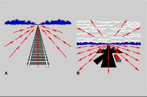
 Sparse Optical Flow vs. Dense Optical Flow. (a) Sparse Optical Flow ... | Download scientific diagram | Sparse Optical Flow vs. Dense Optical Flow. (a) Sparse Optical Flow-Lukas Kanade; (b) Dense Optical Flow-Gunnar Farneback. from publication: Speeding Up Semantic Instance Segmentation by Using Motion Information | Environment perception and understanding represent critical aspects in most computer vision systems and/or applications. State-of-the-art techniques to solve this vision task (e.g., semantic instance segmentation) require either dedicated hardware resources to run or a longer... | Segmentation, Optical Flow and Maps | ResearchGate, the professional network for scientists.
-
 Optical flow models as an open benchmark for radar-based ... - GMD | Apr 9, 2019 ... Figure 2Scheme of the Sparse model. Download. 2.2 The Dense group. The Dense group of models uses, by default, the Dense Inverse ...
-
Any examples for sparse optical flow running on TDA4 DOF ... | Nov 14, 2019 ... This accelerator is primarily a dense optical flow accelerator, meaning that it always computes the flow vectors for every input pixel in the input images.

