Gradient Orientation and Magnitude Explained

• Introduction
• Step-by-Step Guide
• Code Example
• Additional Notes
• Summary
• Conclusion
• References

Image gradients are fundamental building blocks in computer vision, providing crucial information about the structure and edges within an image. This article will delve into the concept of image gradients, explaining how they are calculated, their significance, and their practical applications in various computer vision tasks.

1. Understanding Image Gradients: In simple terms, an image gradient highlights areas of rapid intensity changes in an image. Think of it like outlining the edges of objects.

2. Calculating the Gradient: We typically use operators like Sobel or Scharr to calculate the gradient. These operators use kernels (small matrices) to approximate the image gradient in the horizontal (x) and vertical (y) directions.

   import cv2
   img = cv2.imread('your_image.jpg', cv2.IMREAD_GRAYSCALE)
   sobelx = cv2.Sobel(img, cv2.CV_64F, 1, 0, ksize=5)
   sobely = cv2.Sobel(img, cv2.CV_64F, 0, 1, ksize=5) 

3. Gradient Magnitude: This tells us the "strength" of the edge at a particular pixel. A higher magnitude means a sharper, more defined edge. We calculate it using the Pythagorean theorem:

   gradient_magnitude = cv2.magnitude(sobelx, sobely)

4. Gradient Orientation: This tells us the direction of the edge. Imagine drawing a line perpendicular to the edge – that's your gradient orientation. We calculate it using the arctangent:

   gradient_orientation = cv2.phase(sobelx, sobely, angleInDegrees=True)

5. Applications: Gradient magnitude and orientation are fundamental in computer vision tasks like:

   • Edge Detection: Identifying boundaries of objects.
   • Feature Extraction: Creating descriptors like HOG (Histogram of Oriented Gradients) for object recognition.
   • Image Segmentation: Dividing an image into meaningful regions.

This Python code uses OpenCV and matplotlib libraries to load a grayscale image, calculate its gradient magnitude and orientation using Sobel operators, and then display the original image along with its gradient magnitude, Sobel X, and Sobel Y components in separate subplots.

import cv2
import numpy as np
import matplotlib.pyplot as plt

# **1. Load Image:**
img = cv2.imread('your_image.jpg', cv2.IMREAD_GRAYSCALE)

# **2. Calculate Gradients:**
sobelx = cv2.Sobel(img, cv2.CV_64F, 1, 0, ksize=5)
sobely = cv2.Sobel(img, cv2.CV_64F, 0, 1, ksize=5)

# **3. Gradient Magnitude:**
gradient_magnitude = cv2.magnitude(sobelx, sobely)

# **4. Gradient Orientation:**
gradient_orientation = cv2.phase(sobelx, sobely, angleInDegrees=True)

# **5. Visualization:**
plt.figure(figsize=(12, 6))

plt.subplot(2, 2, 1)
plt.imshow(img, cmap='gray')
plt.title('Original Image')

plt.subplot(2, 2, 2)
plt.imshow(gradient_magnitude, cmap='gray')
plt.title('Gradient Magnitude')

plt.subplot(2, 2, 3)
plt.imshow(sobelx, cmap='gray')
plt.title('Sobel X')

plt.subplot(2, 2, 4)
plt.imshow(sobely, cmap='gray')
plt.title('Sobel Y')

plt.tight_layout()
plt.show()

Explanation:

1. Import Libraries: We import cv2 for OpenCV functions, numpy for numerical operations (although not explicitly used here, it's good practice), and matplotlib.pyplot for plotting.

2. Load Image: We load the image in grayscale using cv2.IMREAD_GRAYSCALE.

3. Calculate Gradients: cv2.Sobel() calculates the Sobel gradients.

   • cv2.CV_64F: Specifies the output data type to handle negative values.
   • 1, 0: Calculates the gradient in the x-direction.
   • 0, 1: Calculates the gradient in the y-direction.
   • ksize=5: Size of the Sobel kernel (5x5 in this case).

4. Gradient Magnitude and Orientation: We use cv2.magnitude() and cv2.phase() to compute these values as explained in the article.

5. Visualization: We use matplotlib to display the original image, gradient magnitude, and Sobel gradients in both x and y directions.

Remember to replace 'your_image.jpg' with the actual path to your image file.

• Choosing the right kernel size: The size of the Sobel or Scharr kernel (e.g., ksize=3, ksize=5) influences the results. Smaller kernels are more sensitive to fine details, while larger kernels provide more smoothing but might miss subtle edges.

• Relationship to derivatives: Mathematically, the Sobel operator approximates the image gradient using derivatives. The x-gradient approximates the derivative in the horizontal direction, and the y-gradient approximates the derivative in the vertical direction.

• Other gradient operators: While Sobel and Scharr are common, other operators like Prewitt, Roberts, and Laplacian of Gaussian (LoG) can also be used to calculate image gradients, each with its own characteristics.

• Gradient magnitude as an edge map: The gradient magnitude image can be thresholded to create a basic edge map. Pixels with gradient magnitudes above a certain threshold are considered edges.

• Gradient orientation for edge direction: The gradient orientation tells us the direction of the edge. For example, an orientation of 0 degrees might indicate a vertical edge, while 90 degrees might indicate a horizontal edge.

• Applications beyond those listed: Image gradients are also used in:

  • Corner detection: Identifying points of rapid change in gradient direction.
  • Image stitching: Aligning images by matching gradient information.
  • Optical flow: Estimating motion between frames using gradient information.

• Understanding the code:

  • The code provided is a basic example. In real-world applications, you'll often need to adjust parameters, apply pre-processing, and post-process the gradient information to suit your specific needs.
  • The cv2.phase() function returns angles in the range of 0 to 360 degrees. You might need to adjust the range or convert to radians depending on your application.

• Further exploration:

  • Explore different gradient operators and their effects on various images.
  • Experiment with different kernel sizes and observe the changes in the gradient results.
  • Implement edge detection or other applications using the calculated gradient information.

This article explains image gradients, a fundamental concept in computer vision. Here's a breakdown:

What are Image Gradients?

• They highlight areas in an image where pixel intensity changes rapidly, essentially outlining edges.

How are they Calculated?

• Operators like Sobel and Scharr, using kernels (small matrices), approximate the gradient in horizontal (x) and vertical (y) directions.
• Python's OpenCV library provides functions for this: cv2.Sobel()

Key Gradient Properties:

• Magnitude: Represents the edge strength at a pixel. Higher magnitude = sharper edge. Calculated using the Pythagorean theorem on x and y gradients.
• Orientation: Indicates the edge direction, calculated using the arctangent of x and y gradients.

Applications in Computer Vision:

• Edge Detection: Finding object boundaries.
• Feature Extraction: Creating descriptors like HOG for object recognition.
• Image Segmentation: Dividing an image into meaningful regions.

By understanding how to compute and utilize image gradients, we unlock a powerful set of tools for analyzing and interpreting visual information in computer vision applications. From basic edge detection to complex object recognition and motion analysis, image gradients provide fundamental insights into the structure and features within images, paving the way for advancements in fields like robotics, medical imaging, and autonomous systems.

• What Is Gradient Orientation and Gradient Magnitude? | Baeldung ... | Explore gradient orientation and magnitude and their applications.
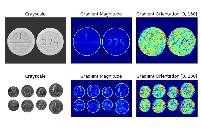• Image Gradients with OpenCV (Sobel and Scharr) - PyImageSearch | In this tutorial, you will learn about image gradients and how to compute Sobel gradients and Scharr gradients using OpenCV’s “cv2.Sobel” function.
• Image gradient - Wikipedia | At each image point, the gradient vector points in the direction of largest possible intensity increase, and the length of the gradient vector corresponds to ...
• imgradient | Calculate Gradient Magnitude and Direction Using Directional Gradients ... Read an image into workspace. I = imread('coins.png');. Calculate the x- and y- ...
• Gradients | Computer Vision | Jun 1, 2020 ... gradient orientation — the direction in which the change in intensity is pointing — and gradient magnitude — which is how strong the change in ...
• Week 5: The image gradient | Step 4: Compute Magnitude at Each Pixel. Page 68. The Gradient Orientation. The gradient orientation: Tells us the direction of greatest intensity change in the.
• Gradient Magnitude - an overview | ScienceDirect Topics | For scalar data, the gradient is a first-derivative measure. As a vector, it describes the direction of greatest change. The normalized gradient is often used ...
• Most accurate visual representation of Gradient Magnitude ... | Sep 12, 2018 ... Also if there are better ways I haven't done below please let me know. # Calculate the Gradient magnitude and direction dX = cv2.Sobel( ...
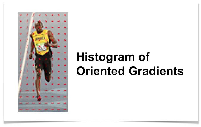• Histogram of Oriented Gradients explained using OpenCV | Histogram of Oriented Gradients (HOG) is a feature descriptor, used for object detection. Read the blog to learn the theory behind it and how it works.