Camera Pose Estimation from Homography of 4 Points

• Introduction
• Step-by-Step Guide
• Code Example
• Additional Notes
• Summary
• Conclusion
• References

In this tutorial, we'll explore how to determine the pose of a camera relative to a known planar surface using homography decomposition in computer vision. This technique is particularly useful in applications like augmented reality, robot navigation, and 3D reconstruction. We'll break down the process into four key steps, guiding you through the code and explaining the underlying concepts.

1. Find point correspondences: Identify at least four corresponding 2D points in your image and their known 3D world coordinates on the plane.

   # Example 2D image points
   image_points = np.array([[100, 50], [200, 80], [150, 150], [250, 180]], dtype=np.float32)
   
   # Example 3D world points on the plane (assuming z=0 for simplicity)
   world_points = np.array([[0, 0, 0], [1, 0, 0], [0, 1, 0], [1, 1, 0]], dtype=np.float32)

2. Calculate the homography matrix: Use OpenCV's findHomography function to estimate the homography matrix (H) that maps the world points to the image points.

   H, _ = cv2.findHomography(world_points, image_points)

3. Decompose the homography matrix: Extract the camera pose (rotation and translation) from the homography matrix using OpenCV's decomposeHomographyMat. This function returns multiple possible solutions, so you'll need to select the most appropriate one based on your scene knowledge.

   num_solutions, rotations, translations, normals = cv2.decomposeHomographyMat(H, camera_matrix)
   
   # Select the best solution based on your scene
   best_solution_index = ... 
   R = rotations[best_solution_index]
   t = translations[best_solution_index]

4. Refine the pose (optional): For improved accuracy, you can refine the estimated pose using iterative methods like solvePnP with the original 3D-2D correspondences.

   _, rvec, tvec = cv2.solvePnP(world_points, image_points, camera_matrix, dist_coeffs)
   
   # Convert rotation vector to rotation matrix
   R, _ = cv2.Rodrigues(rvec)

Note: camera_matrix and dist_coeffs represent the camera's intrinsic parameters and distortion coefficients, respectively. You need to calibrate your camera beforehand to obtain these parameters.

This Python code estimates the pose of a camera relative to a planar surface. It uses a set of corresponding 2D image points and 3D world points on the plane. The code first calculates the homography matrix and then decomposes it to obtain possible rotation and translation solutions. After selecting the best solution, it refines the pose using the SolvePnP algorithm. Finally, it prints the estimated rotation matrix and translation vector of the camera.

import cv2
import numpy as np

# Camera parameters (replace with your calibrated values)
camera_matrix = np.array([[1000, 0, 500],
                         [0, 1000, 300],
                         [0, 0, 1]], dtype=np.float32)
dist_coeffs = np.zeros((5,), dtype=np.float32)

# 2D image points
image_points = np.array([[100, 50], [200, 80], [150, 150], [250, 180]], dtype=np.float32)

# 3D world points on the plane (assuming z=0)
world_points = np.array([[0, 0, 0], [1, 0, 0], [0, 1, 0], [1, 1, 0]], dtype=np.float32)

# Calculate the homography matrix
H, _ = cv2.findHomography(world_points, image_points)

# Decompose the homography matrix
num_solutions, rotations, translations, normals = cv2.decomposeHomographyMat(H, camera_matrix)

# Select the best solution (replace with your criteria)
best_solution_index = 0  
R = rotations[best_solution_index]
t = translations[best_solution_index]

# Refine the pose using solvePnP
_, rvec, tvec = cv2.solvePnP(world_points, image_points, camera_matrix, dist_coeffs)

# Convert rotation vector to rotation matrix
R, _ = cv2.Rodrigues(rvec)

# Print the estimated camera pose
print("Rotation matrix (R):\n", R)
print("Translation vector (t):\n", tvec)

Explanation:

1. Camera Parameters: Replace the placeholder values for camera_matrix and dist_coeffs with the intrinsic parameters and distortion coefficients obtained from your camera calibration.
2. Point Correspondences: The code defines example 2D image points and their corresponding 3D world coordinates on the plane. Ensure these points are accurate for your specific setup.
3. Homography Estimation: cv2.findHomography calculates the homography matrix that maps the world points to the image points.
4. Homography Decomposition: cv2.decomposeHomographyMat extracts the possible rotation matrices, translation vectors, and normal vectors from the homography matrix. You need to select the most appropriate solution based on your scene knowledge.
5. Pose Refinement: cv2.solvePnP refines the estimated pose using an iterative optimization method. This step can improve accuracy, especially if the initial homography estimation is noisy.
6. Output: The code prints the final estimated rotation matrix (R) and translation vector (tvec) representing the camera pose relative to the plane.

Remember to adapt the code to your specific application, including selecting the appropriate solution from decomposeHomographyMat and potentially defining criteria for choosing the best solution.

• Planar Assumption: This method relies heavily on the fact that the world points lie on a plane. If this assumption doesn't hold, the estimated pose will be inaccurate.
• Minimum Points: You need at least four non-collinear point correspondences to compute the homography matrix. Using more points generally improves robustness to noise.
• Solution Ambiguity: Decomposing the homography matrix often yields multiple possible solutions for rotation and translation. Selecting the correct solution requires additional scene knowledge or constraints. For instance:
  • Normal Vector: The normals output from decomposeHomographyMat provides the surface normal of the plane. You can use this to discard solutions where the normal points in the wrong direction relative to the camera.
  • Scene Constraints: If you have prior information about the camera's position or orientation (e.g., it's roughly upright), you can use this to eliminate unrealistic solutions.
• Pose Refinement: The optional pose refinement step using solvePnP is highly recommended as it can significantly improve accuracy by minimizing reprojection errors.
• Units: The units of the translation vector (tvec) depend on the units used for the 3D world points. Ensure consistency in your units throughout the process.
• Applications: This technique has various applications, including:
  • Augmented Reality: Superimposing virtual objects onto real-world scenes.
  • Robot Navigation: Localizing a robot with respect to a known planar landmark.
  • 3D Reconstruction: Building 3D models of objects or environments from images.

Code Considerations:

• Error Handling: The code assumes successful execution of OpenCV functions. In a real-world application, you should include error handling to gracefully manage potential failures.
• Solution Selection Criteria: The code uses a placeholder (best_solution_index = 0) for selecting the best solution. You'll need to implement your own criteria based on your specific application and scene knowledge.
• Visualization: Consider visualizing the estimated camera pose and the reprojected 3D points on the image to verify the results and debug any issues.

This text describes a method for estimating the camera pose (position and orientation) relative to a known planar object in an image.

Here's a breakdown of the process:

1. Establish Correspondences: Identify at least four 2D points in your image and their corresponding 3D world coordinates on the plane. These points act as anchors connecting the image to the real world.

2. Compute Homography: Utilize the OpenCV function findHomography to calculate the homography matrix (H). This matrix encapsulates the transformation that maps the 3D plane to the 2D image.

3. Extract Camera Pose: Decompose the homography matrix using decomposeHomographyMat to obtain the camera's rotation (R) and translation (t) relative to the plane. This function may provide multiple solutions, requiring you to select the most plausible one based on your scene understanding.

4. Optional Refinement: Enhance the accuracy of the estimated pose by employing iterative techniques like solvePnP with the original 3D-2D point correspondences. This step helps refine the initial estimate.

Important Considerations:

• Camera Calibration: This method necessitates prior camera calibration to obtain the camera matrix and distortion coefficients, which are crucial for accurate pose estimation.
• Solution Selection: Carefully analyze the multiple solutions provided by decomposeHomographyMat and choose the one that aligns best with your scene knowledge.

By following these steps, you can effectively estimate the camera pose relative to a planar target in an image.

This process outlines a robust method for determining the camera pose in relation to a planar target using homography decomposition. By accurately identifying corresponding points, calculating the homography matrix, and refining the solution, we can achieve precise camera pose estimation. This technique proves valuable in various applications, including augmented reality, robot navigation, and 3D reconstruction, contributing to advancements in computer vision and related fields.

• Basic concepts of the homography explained with code - OpenCV | Camera pose estimation from coplanar points for augmented ... This demo shows you how to compute the homography transformation from two camera poses.
• python - OpenCV - homographic conversion on point used for matrix ... | Jul 5, 2023 ... OpenCV: use solvePnP to determine homography · 49 · Computing camera pose with homography matrix based on 4 coplanar points · 2 · Opencv ...
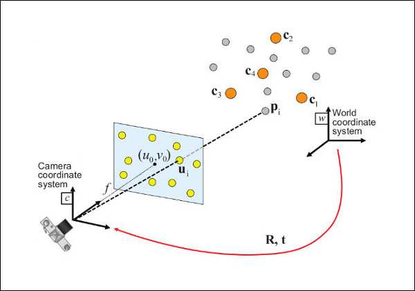• Perspective-n-Point (PnP) pose computation - OpenCV | The solvePnP and related functions estimate the object pose given a set of object points, their corresponding image projections, as well as the camera intrinsic ...
• Finding the camera orientation from a homography, opencv - Stack ... | Dec 12, 2012 ... Computing camera pose with homography matrix based on 4 coplanar points. Related. 6 · Calculating homography matrix using arbitrary known ...
• Obtaining accurate pose of camera facing a plane : r/computervision | Posted by u/jlKronos01 - 6 votes and 44 comments
• opencv - Determine camera rotation between two 360x180 ... | Jul 25, 2012 ... To calculate the camera pose you need to find homography ... Computing camera pose with homography matrix based on 4 coplanar points.
• Turning ArUco marker in parallel with camera plane - OpenCV Q&A ... | Mar 30, 2017 ... ... compute the homography matrix from the camera displacement. ... How the homography can be useful? Camera pose estimation with coplanar points ...
• Pose Estimation Based on Four Coplanar Point Correspondences | 4) Set the camera's intrinsic matrix equal to identity. Hence the ... 7) Computer the homography matrix H using the algorithm presented in section ...
• Finding 3D coordinate when all 3 coordinates can vary in the object ... | Feb 25, 2014 ... I have the 3D coordinates of 4 coplanar points of my target in ... compute-camera-pose-from-homography-matrix. to a 3D plane requires at ...