OpenCV HOG Feature Extraction Tutorial

• Introduction
• Step-by-Step Guide
• Code Example
• Additional Notes
• Summary
• Conclusion
• References

In computer vision, extracting meaningful features from images is crucial for tasks like object detection and image recognition. The Histogram of Oriented Gradients (HOG) is a powerful feature descriptor that effectively captures the distribution of gradient orientations within an image. This article provides a step-by-step guide on how to extract HOG features from images using Python and the OpenCV library. We'll cover loading an image, converting it to grayscale, creating a HOG descriptor, computing HOG features, and visualizing the results. Additionally, we'll briefly demonstrate how these features can be used for tasks like training a Support Vector Machine (SVM) classifier.

1. Import necessary libraries:

import cv2

2. Load an image:

image = cv2.imread('image.jpg')

3. Convert the image to grayscale:

gray = cv2.cvtColor(image, cv2.COLOR_BGR2GRAY)

4. Create a HOG descriptor object:

hog = cv2.HOGDescriptor()

5. Compute HOG features:

features = hog.compute(gray)

6. (Optional) Visualize HOG features:

from skimage import feature
import matplotlib.pyplot as plt

hog_image = feature.hog(gray, visualize=True)
plt.imshow(hog_image, cmap='gray')
plt.show()

7. Use HOG features for object detection or other tasks:

# Example: Train an SVM classifier
from sklearn.svm import SVC

clf = SVC(kernel='linear')
clf.fit(features.reshape(1, -1), [1])  # Train with a single positive sample

Explanation:

• HOG (Histogram of Oriented Gradients) is a feature descriptor that captures the distribution of gradient orientations in an image.
• We first convert the image to grayscale and create a HOG descriptor object.
• The compute() method extracts HOG features from the image.
• We can visualize the HOG features using the skimage.feature.hog() function.
• The extracted features can be used for various tasks, such as object detection, by training a machine learning model like SVM.

This Python code demonstrates how to extract Histogram of Oriented Gradients (HOG) features from an image using OpenCV and scikit-image. It loads an image, converts it to grayscale, and computes HOG features using a HOG descriptor. The code then visualizes the HOG features using matplotlib. Finally, it shows a placeholder example of training a Support Vector Machine (SVM) classifier with the extracted features, highlighting that in a real application, a labeled dataset would be used for training.

import cv2
from skimage import feature
import matplotlib.pyplot as plt
from sklearn.svm import SVC

# Load an image
image = cv2.imread('image.jpg')

# Convert the image to grayscale
gray = cv2.cvtColor(image, cv2.COLOR_BGR2GRAY)

# Create a HOG descriptor object
hog = cv2.HOGDescriptor()

# Compute HOG features
features = hog.compute(gray)

# Visualize HOG features
hog_image = feature.hog(gray, visualize=True)
plt.imshow(hog_image[1], cmap='gray')
plt.title('HOG Features')
plt.show()

# Example: Train an SVM classifier (using placeholder data)
clf = SVC(kernel='linear')
clf.fit(features.reshape(1, -1), [1])  # Train with a single positive sample

# In a real application, you would train the classifier with a dataset
# of positive and negative samples.

Explanation:

1. Import Libraries: We import cv2 for image processing, skimage.feature for HOG feature visualization, matplotlib.pyplot for plotting, and sklearn.svm for the SVM classifier.
2. Load and Preprocess Image: We load the image using cv2.imread() and convert it to grayscale using cv2.cvtColor().
3. Create HOG Descriptor: We create a cv2.HOGDescriptor() object with default parameters.
4. Compute HOG Features: We extract HOG features from the grayscale image using hog.compute().
5. Visualize HOG Features: We use skimage.feature.hog() to visualize the HOG features. The visualize=True argument returns the HOG image, which we display using matplotlib.pyplot.
6. Train SVM Classifier (Placeholder): This section demonstrates how to train an SVM classifier using the extracted HOG features. Note: This is a simplified example using placeholder data. In a real application, you would train the classifier with a labeled dataset of positive and negative samples.

To use this code:

• Replace 'image.jpg' with the path to your image file.
• Make sure you have the required libraries installed (opencv-python, scikit-image, matplotlib, scikit-learn). You can install them using pip:

  pip install opencv-python scikit-image matplotlib scikit-learn

This code will extract HOG features from your image, visualize them, and demonstrate a basic example of training an SVM classifier. Remember that for real-world object detection tasks, you need a proper dataset and more robust training procedures.

• HOG Descriptor Parameters: The cv2.HOGDescriptor() object can be initialized with various parameters to customize the HOG feature extraction process. These parameters include:

  • winSize: Size of the detection window (usually the same as the image size).
  • blockSize: Size of the blocks into which the image is divided.
  • blockStride: Step size for sliding the block window.
  • cellSize: Size of the cells within each block.
  • nbins: Number of orientation bins for the histogram.

• Feature Vector Dimensionality: The dimensionality of the extracted HOG feature vector depends on the chosen parameters and the image size. It's calculated as: (Number of blocks in x-direction) * (Number of blocks in y-direction) * (Number of cells per block) * (Number of orientation bins)

• Normalization: HOG features are typically normalized to improve their robustness to changes in illumination. Common normalization techniques include L2-norm, L2-Hys (L2-norm followed by clipping and renormalization), and L1-sqrt (L1-norm followed by square root).

• Applications of HOG Features:

  • Object Detection: HOG features are widely used in object detection algorithms, particularly for pedestrian detection.
  • Image Recognition: They can be used as features for image classification tasks.
  • Action Recognition: HOG features computed over video frames can be used to recognize human actions.

• Advantages of HOG Features:

  • Robustness to Illumination Changes: Normalization techniques make HOG features less sensitive to variations in lighting conditions.
  • Invariance to Geometric Transformations: HOG features are relatively invariant to small geometric transformations like translation and rotation.
  • Computational Efficiency: HOG feature extraction is computationally efficient, making it suitable for real-time applications.

• Limitations of HOG Features:

  • Sensitivity to Background Clutter: HOG features can be affected by complex backgrounds.
  • Not Scale-Invariant: HOG features are not inherently scale-invariant, so multi-scale detection is often required.

This code snippet demonstrates how to extract HOG (Histogram of Oriented Gradients) features from an image using OpenCV and Python.

Here's a breakdown:

1. Load Image: The code loads an image named "image.jpg" using OpenCV's imread() function.
2. Convert to Grayscale: The image is converted to grayscale using cvtColor(), as HOG operates on grayscale images.
3. Create HOG Descriptor: A HOG descriptor object is created using cv2.HOGDescriptor(). This object holds the parameters for HOG feature extraction.
4. Compute HOG Features: The compute() method of the HOG descriptor object extracts HOG features from the grayscale image.
5. (Optional) Visualize Features: The code provides an optional step to visualize the extracted HOG features using skimage.feature.hog() and matplotlib.
6. Utilize Features: The extracted HOG features can be used for various computer vision tasks, such as object detection. The code provides an example of training a Support Vector Machine (SVM) classifier using the extracted features.

In essence, this code demonstrates a simple pipeline for:

• Loading an image.
• Extracting meaningful HOG features that capture gradient information.
• Optionally visualizing these features.
• Utilizing the features for further image processing tasks like object detection.

This code snippet provides a practical illustration of how to extract HOG features from images using OpenCV in Python. By understanding the basic principles and implementation details presented here, you can leverage the power of HOG features for various computer vision applications, including object detection and image recognition. Remember that fine-tuning HOG parameters and employing robust machine learning techniques are crucial for achieving optimal performance in real-world scenarios.

• Extracting Histogram of Gradients with OpenCV ... | Besides the feature descriptor generated by SIFT, SURF, and ORB, as in the previous post, the Histogram of Oriented Gradients (HOG) is another feature descriptor you can obtain using OpenCV. HOG is a robust feature descriptor widely used in computer vision and image processing for object detection and recognition tasks. It captures the distribution of […]
• Get HOG image features from OpenCV + Python? - Stack Overflow | May 22, 2011 ... In python opencv you can compute hog like this: import cv2 hog = cv2.HOGDescriptor() im = cv2.imread(sample) h = hog.compute(im).
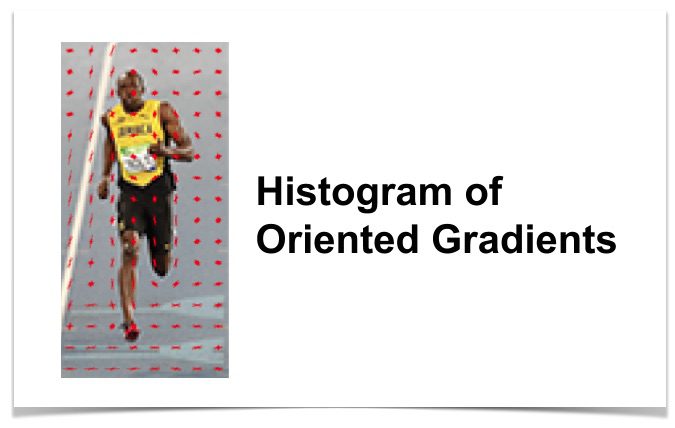• Histogram of Oriented Gradients explained using OpenCV | Histogram of Oriented Gradients (HOG) is a feature descriptor, used for object detection. Read the blog to learn the theory behind it and how it works.
• Comparing two HOG descriptors vectors - OpenCV Q&A Forum | Nov 4, 2012 ... http://stackoverflow.com/questions/11626140/extracting-hog-features-using-opencv. they just do a hog-to-hog distance accumulating the error..
• How to reduce extract image feature time? - Python - OpenCV | Hi everyone, I have just learned about computer vision. Currently, i am processing a problem about image classification. I used HoG to extract features from images, but it takes a very long time whenever i run it. Is there anyway to reduce the time run it because my dataset is very large (about 15k images). And HoG extracts an image into a (1, 16740) vector dimension. Here is the code i uses to extract features: def calc_hog(imgPath): img = cv2.imread(imgPath) gray = cv2.cvtColor(img,...
• How to match 2 HOG for object detection? - OpenCV Q&A Forum | Jul 28, 2012 ... I have already implemenet SIFT and ORB for detection. Now I would like to add HOG matching. I can extract HOG feature by doing: Mat image( ...
• After Hog feature extraction do I need to use StandardScaler before ... | Hello, I am a beginner in the field of image processing and machine learning und I hope I’m here in the right forum. It’s about training an SVM (support vector machine) with hog features from images which are reduced by PCA (principal component analysis). The Hog features are extracted as follows: from skimage import feature ... feat = feature.hog(image, orientations=12, pixels_per_cell=(4,4), cells_per_block=(2,2), block_norm='L2_Hys', transform_sqrt=True) ... The hog feature vectors conta...
• How to predict HOG features each frame with trained SVM classifier ... | Apr 4, 2018 ... type() == 5 in function predict". I made sure my extracted features are float32 numpy arrays. If someone could help me find out why this is ...
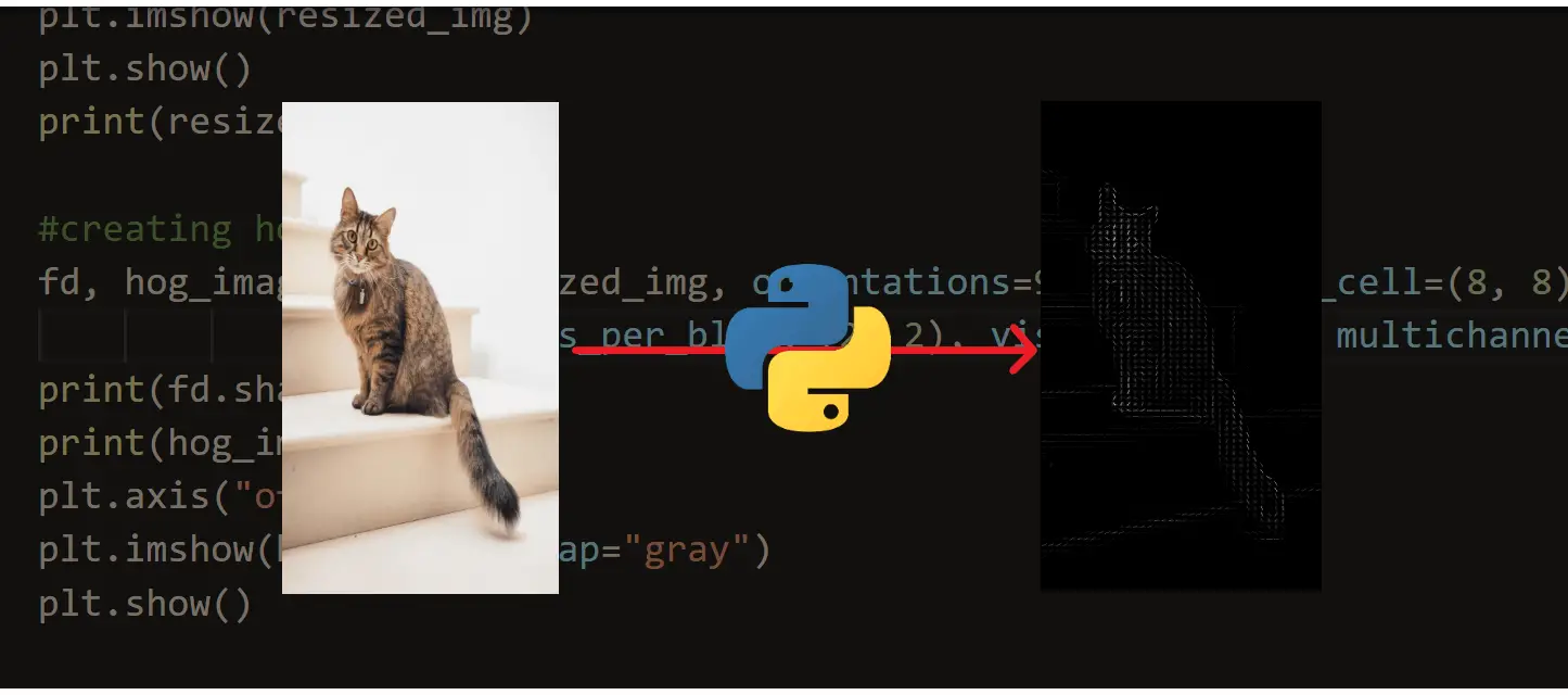• How to Apply HOG Feature Extraction in Python - The Python Code | Learn how to use scikit-image library to extract Histogram of Oriented Gradient (HOG) features from images in Python.